Given a community abundance matrix, compute the species abundance distribution as rank abundance curve.
rad(x, remove.zeros = TRUE, fit.neutral = FALSE, fit.rad = FALSE,
  fit.distrib = FALSE, fit.N = nrow(x), sample.index = NA,
  plot = TRUE, header = "")
Arguments
| x | community matrix with species as rows, samples as columns and non-negative integers as entries |
|---|---|
| remove.zeros | if true, zeros in the species abundance distribution curve are discarded |
| fit.neutral | assess the fit of the neutral model with function theta.prob from the untb R package |
| fit.rad | (optional) fit different RAD models using vegan's radfit function. If selected, fit.distrib is ignored and if plot is true, vegan's plot function for RAD curves is used. |
| fit.distrib | (optional) select the best-fitting distribution for the RAD by comparing normal, lognormal, gamma, negative binomial and Poisson distribution using MASS function fitdistr |
| fit.N | (optional) number of samples drawn from the distribution to be fitted (defaults to the number of species in x after filtering of zeros) |
| sample.index | (optional) the sample index for which species abundance distribution is computed, if not provided, the mean across samples is taken |
| plot | plot the RAD curve |
| header | add the header to the title of the plot |
Value
the RAD parameters are returned, if fit.neutral is true, the probability of the biodiversity parameter theta is returned, if fit.rad or fit.distrib is true, the results of distribution fitting are also returned (distrib, score [log-likelihood for fit.distrib and AIC for fit.rad], params and fitted.rad)
Details
Please provide species abundances as counts (scale and round if necessary). Note that for fit.rad, Null is the broken stick distribution. A vector of species abundances can be provided as well.
Examples
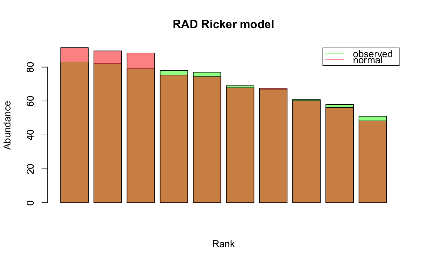
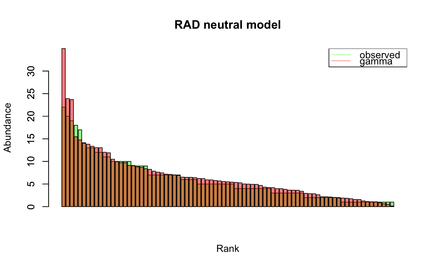
#> [1] "Adjusting connectance to 0.02" #> [1] "Initial edge number 100" #> [1] "Initial connectance 1" #> [1] "Number of edges removed 89" #> [1] "Final connectance 0.0111111111111111" #> [1] "Final connectance: 0.0111111111111111"ts.ricker=round(ts.ricker*1000) # scale to integers rad.out.ricker=rad.fit.ricker=rad(ts.ricker, fit.distrib = TRUE, header="Ricker model")#> [1] "Selected distribution: normal" #> [1] "Fitting score: -37.6939444195898" #> [1] "Fitting parameters:" #> mean sd #> 70.50000 10.49047ts.hubbell=simHubbell(N = 100, M = 100, I = 500, d = 1, tskip=500, tend=1500) rad.out.hubbell=rad.fit.hubbell=rad(ts.hubbell, fit.distrib = TRUE, header="neutral model")#> [1] "Removing 19 species with zero abundance." #> [1] "Selected distribution: gamma" #> [1] "Fitting score: -220.85263492036" #> [1] "Fitting parameters:" #> shape rate #> 1.620168 0.271144