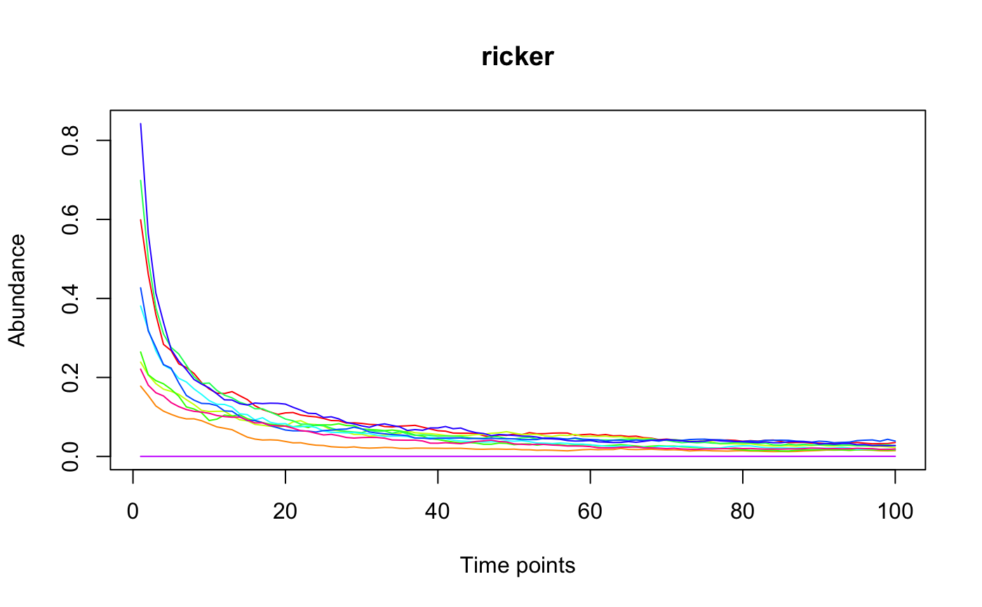
The Ricker model is a discrete version of the generalized Lotka-Volterra model and is implemented here as proposed by Fisher and Mehta in PLoS ONE 2014.
ricker(N, A, K = rep(0.1, N), y = runif(N), sigma = 0.05,
  K.trend = NA, tend = 100, death.t = NA, tskip = 0,
  explosion.bound = 10^8, perturb = NULL)
Arguments
| N | number of species |
|---|---|
| A | interaction matrix |
| K | a vector of carrying capacities |
| y | initial abundances |
| sigma | noise level, if set to a non-positive value, no noise is added |
| K.trend | a vector of positive or negative carrying capacity percentages specified between 0 and 1 |
| tend | number of time points |
| death.t | species with abundance below this value are killed (abundance is set to 0) |
| tskip | number of initial time points to skip (to skip the transient) |
| explosion.bound | boundary for explosion |
| perturb | a perturbation object |
Value
a matrix with species abundances as rows and time points as columns
Details
If an explosion occurs, -1 is returned. An explosion is reported if any species crosses the explosion bound. To avoid explosions, decrease the number of interactions in the interaction matrix and/or increase the number of negative interactions in the interaction matrix. K.trend contains carrying capacity percentages (from the original carrying capacity) that are added to each species' current carrying capacity in each time step. K.trend allows to simulate an environmental trend. Negative carrying capacities are set to zero. If both a perturbation and K.trend are specified, the perturbation is carried out first.
References
Fisher & Mehta (2014). Identifying Keystone Species in the Human Gut Microbiome from Metagenomic Timeseries using Sparse Linear Regression. PLoS One 9:e102451
See also
glv for the generalized Lotka Volterra model
Examples
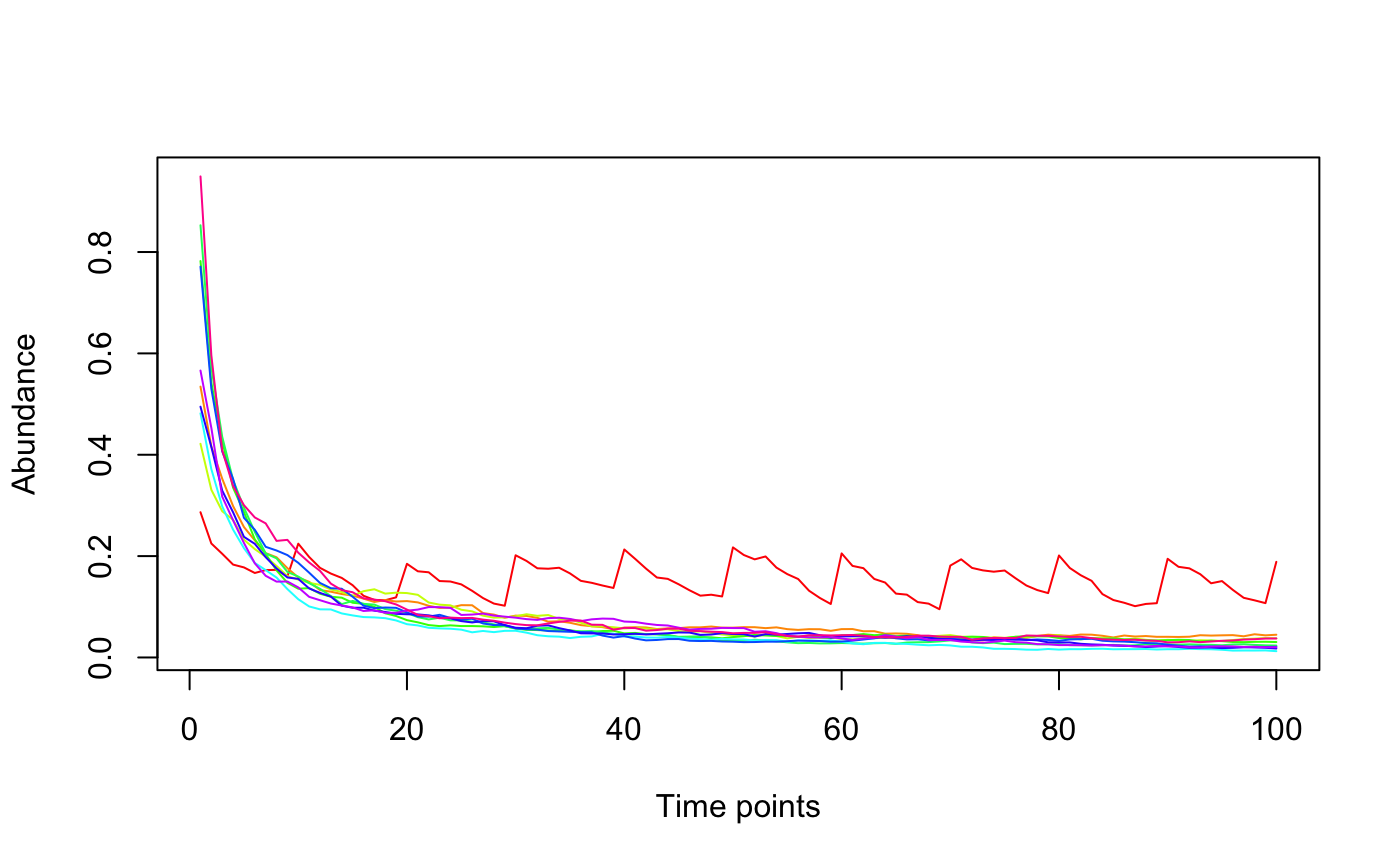
#> [1] "Adjusting connectance to 0.02" #> [1] "Initial edge number 100" #> [1] "Initial connectance 1" #> [1] "Number of edges removed 89" #> [1] "Final connectance 0.0111111111111111" #> [1] "Final connectance: 0.0111111111111111"per=perturbation(times=seq(10,100,10),durations=rep(1,10),numberchanges=c(0.1,rep(0,9))) tsplot(ricker(10,generateA(10),K=rep(0.01,10),perturb=per))#> [1] "Adjusting connectance to 0.02" #> [1] "Initial edge number 100" #> [1] "Initial connectance 1" #> [1] "Number of edges removed 89" #> [1] "Final connectance 0.0111111111111111" #> [1] "Final connectance: 0.0111111111111111"

